Sales Forecasting (1) From Tree Models to Chronos

Sales forecasting is hard.

The day of the week matters. So do the season, the weather and promotions. When a seller changes their product line one day, half the value of their past sales disappears. Much of this never lands in the data at all.

So in commerce it usually counts as inventory and logistics work.

For a fintech that lends against sales, it is a different story.

A seller’s future sales are the source of repayment. Forecasting moves to the centre of limits, repayment and risk management.

This series is about how to build that forecast. This part covers what to predict and which model to use, and the next part opens up the transformer.

1. What forecasting does in revenue-based financing

Revenue-based financing is simple in structure. You lend by looking at a seller’s sales flow, and repayment comes out of sales too.

Shopify Capital is the familiar example, where a fixed share of daily sales goes to repayment automatically (Shopify). Good days repay more, slow days repay less.

The limit is the first place a forecast gets used. How much a seller will sell over the next few months caps how much you can lend.

Repayment time depends on the forecast as well. How long it takes to repay at a given share of daily sales is decided by the path of sales.

After the loan goes out, the forecast becomes an early warning. You want to catch sellers whose sales are starting to turn down.

But these three want slightly different forecasts.

For the limit, the question is how much a seller sells when things go badly: the lower end of the distribution. For repayment time, an ordinary sales path is enough. For early warning, direction matters more than level.

So before choosing a model, decide what to predict.

2. How it differs from forecasting stock prices

Many people hear “time series forecasting” and think of stock prices. Sales behave quite differently.

A stock price is close to a random walk, so there is little to add beyond its past, and what you add carries a weak signal.

Sales have structure. There are weekdays, seasons and promotions. Above all, there are many covariates to consider.

Covariates split by when their values become known.

Category, tenure and region don’t change over time: static covariates. Return rates, ratings, review counts and visits are known only afterwards. The calendar, public holidays and promotions already on the schedule are known in advance, future values included.

The distinction matters for one reason.

In the forecast window, the model can only use the static covariates and the last kind.

What goes into a sales forecast

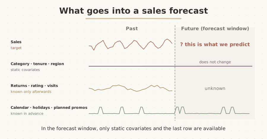
A stock forecast has little more than the first row.

Then there is the seller side. Hundreds of thousands of sellers means hundreds of thousands of series, with scale ranging from tens of thousands of won a day to hundreds of millions.

Small sellers often have zero-sales days (intermittent demand). A newly onboarded seller has two or three months of history. Change the product line and past sales stop explaining the future.

One model has to handle all of these uneven series at once. That is the real reason sales forecasting is hard.

3. What to predict

The amount itself

The most intuitive choice is to predict future sales in currency. You can use the result directly. A 30-day forecast goes straight into the limit calculation, and daily point forecasts add up to a monthly one.

Scale is the problem. Sellers differ by a factor of a thousand, so a loss measured in currency pulls training towards the big sellers. Errors grow with scale too (heteroscedasticity).

A log transform helps. But predicting in log space and transforming back lands near the median rather than the mean, a retransformation bias.

A tree model predicting the raw amount can’t produce values larger than it saw in training. More on that in section 5.

There is a flip side.

For a lender, a big seller’s error really is more money, so being pulled towards big sellers is not purely bad. The M5 competition on Walmart sales used a metric weighted by sales value too.

Whether to erase or keep the scale differences depends on where your losses come from.

The growth rate

The second choice is to predict how much sales rise or fall against the last period. It is scale-free, so sellers become comparable.

Once trend is removed the series gets closer to stationary, which is easier for a model to learn. If catching sellers in decline is the goal, it is the most direct option.

But it is undefined when the base is zero.

A seller who sold nothing yesterday and ₩10,000 today has grown by what percentage? Infinity. With small, intermittent sellers, this blows up often.

Multi-period forecasts are a problem too. Turning growth rates back into amounts means multiplying them, and errors compound. There is asymmetry as well: −50% followed by +50% doesn’t get you back where you started.

Log ratios fix the asymmetry, but the zero problem stays. So in practice people often aggregate periods to avoid zeros, as in “next 30 days’ total ÷ last 30 days’ total”.

The distribution

The third choice is to predict a distribution rather than a single value, usually as quantiles. “Next 30 days’ sales: P10 ₩46M, P50 ₩53M, P90 ₩61M.”

This matters most in lending, because the losses come from the lower end. Set a limit on a mean forecast and actual sales come in below it about half the time.

A distribution lets you draw a line: the amount a seller sells even when things go badly. You can also treat a volatile seller differently from a steady one with the same mean.

The cost is harder evaluation and operation. There is no single right answer, so you need pinball loss or CRPS, and a separate coverage check: do 10% of outcomes really fall below P10?

Train one model per quantile and you can get crossing, with P10 above P50. The tails have less data and are less stable. And there is one more trap the next part covers in detail. Daily quantiles don’t add up to a monthly quantile.

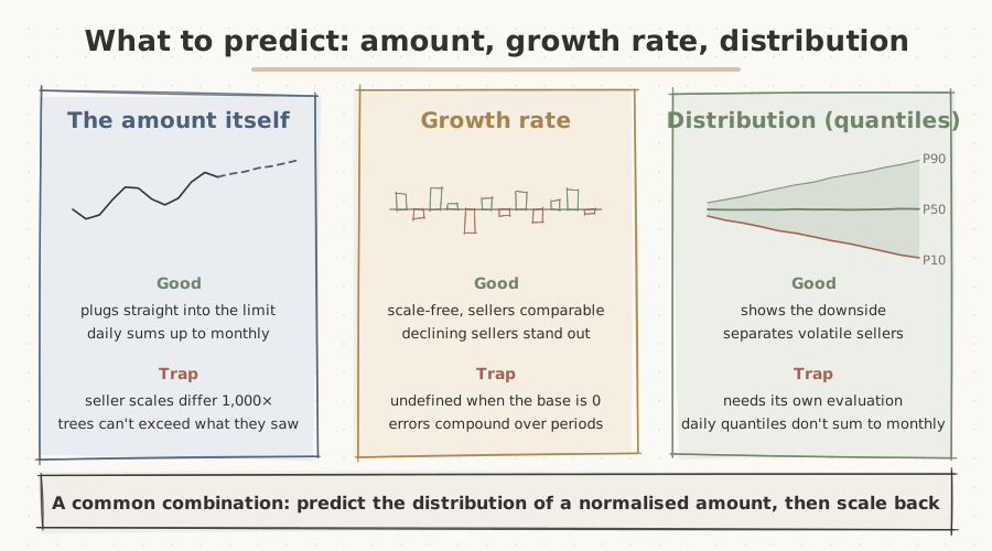
What to predict: amount, growth rate, distribution

Each has its uses, and each has a trap.

Scale and output form are separate choices

These three are not really points on one line.

Amount versus ratio is a question of scale. Point versus distribution is a question of output form. So in practice people combine them: predict the distribution of a normalised amount per seller, then scale it back.

That is exactly what the Chronos models later in this post do. Normalise each series, predict quantiles in the normalised space, then map back to the original scale.

4. The quantile you use is set by cost

Once you predict a distribution, the next question follows. Which quantile sets the limit?

P10 or P20? It is often decided by gut feel, but the answer is known.

Pinball loss, the loss function of quantile regression, works like this. At quantile τ, when the actual value is above the prediction the penalty is weighted by τ, and when it is below, by 1−τ.

That is exactly the newsvendor problem from inventory management.

Stock too many papers and you pay for the leftovers. Stock too few and you pay in lost sales. The ratio of those two costs sets the optimal order.

For lending, the two costs look like this. Overestimating sales and lending too much is the over-lending cost. Underestimating and lending too little (lost interest, sellers who leave for a competitor) is the under-lending cost. The quantile that minimises expected cost is the under-lending cost divided by the sum of the two.

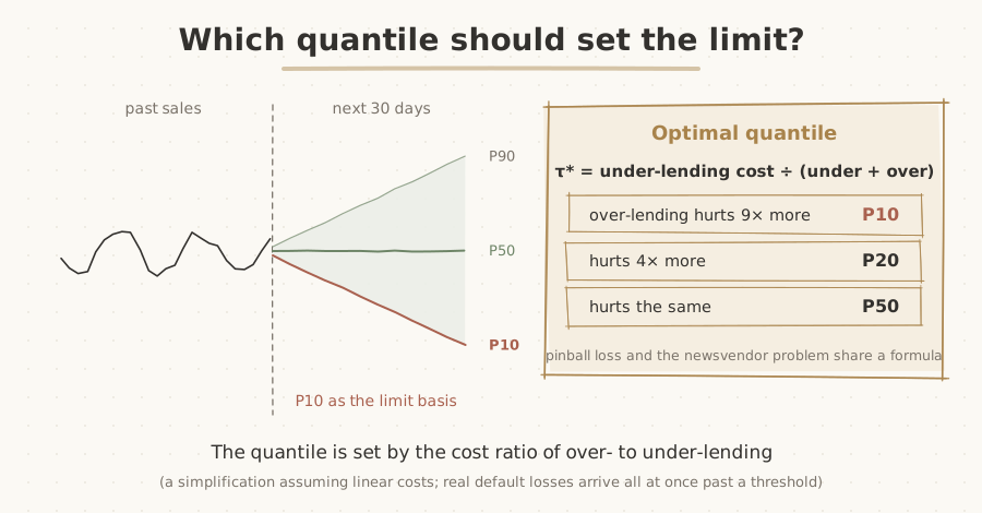
Which quantile should set the limit?

Setting limits at P10 means treating over-lending as nine times as painful as under-lending.

Read it backwards and it gets more interesting.

Using P10 means you have judged one unit of over-lending to hurt nine times as much as one unit of under-lending. Put that number on the table and the risk team and the business team can argue about quantiles in terms of cost rather than instinct.

It is a simplification, of course. Real default losses don’t scale linearly with the sales shortfall; past a threshold they arrive all at once.

Still, it is a useful place to start.

5. Tree models, still the strongest baseline

The workhorse of sales forecasting is still gradient-boosted trees such as LightGBM. In the 2020 M5 competition, forecasting 42,840 Walmart series, most of the top entries used LightGBM.

The trick is turning the series into a table, with one row per cutoff date.

Add lags and rolling statistics from past sales. Add the calendar and planned promotions for the forecast window, last period’s return rate and rating, and static attributes like category. A single global model across all sellers is the usual choice.

Quantiles take one parameter. LightGBM uses objective="quantile" with alpha. XGBoost takes reg:quantileerror with quantile_alpha, several quantiles at once. CatBoost uses Quantile:alpha=0.1 or MultiQuantile:alpha=0.1,0.5,0.9.

M5 even had a separate uncertainty track asking for nine quantiles.

import lightgbm as lgb
import numpy as np

# y = next 30 days' sales / last 30 days' sales  (a scale-free ratio target)
quantiles = [0.1, 0.5, 0.9]
pred = {}
for q in quantiles:
    m = lgb.LGBMRegressor(objective="quantile", alpha=q,
                          n_estimators=400, learning_rate=0.05, num_leaves=31)
    m.fit(X_train, y_train, categorical_feature=["category"])
    pred[q] = m.predict(X_valid)

P = np.sort(np.column_stack([pred[q] for q in quantiles]), axis=1)  # fix quantile crossing
limit_basis = P[:, 0] * past30_valid   # P10 ratio × last 30 days' sales = limit basis

I ran this on synthetic data: 300 sellers, two years of daily sales with promotions and return rates attached.

I trained a P10 model, and in the later validation period 13.7% of actual values fell below P10. P90 had narrowed inward to 86.8% too.

Even when you train for a quantile, coverage drifts once the period changes. So the quantile used for limits needs a separate calibration step on recent data.

Extrapolation was more dramatic.

I fed a model trained on the raw amount, rather than the ratio, sellers at 1×, 3× and 10× the training maximum. How much did the forecast grow? Not by a single won.

Any input larger than the largest training value falls into the same leaf.

It is like measuring height with a ruler whose markings stop at the tallest person you have met.

So the faster a seller grows, the more they are underestimated. Switch the target to a ratio and the problem goes away. This is what I meant in section 3 about the choice of target carrying into the choice of model.

Tree models take any number of heterogeneous covariates as columns. They are fast, and SHAP makes them easy to explain.

Their weakness is that they don’t see the series directly.

Everything about order has to be hand-built as lags and rolling statistics. Forecasting several days ahead means one model per day (the direct approach) or feeding predictions back in (the recursive approach, where errors accumulate).

Train one model per quantile and crossing can appear. It didn’t in the experiment above, but it is worth checking every time.

6. Time series transformers, from TFT to Chronos

There are two roads to a transformer.

One is a task-specific model trained from scratch on your own data. The standard example is Google’s TFT (Temporal Fusion Transformer), and its structure fits sales forecasting closely.

It takes the three kinds of covariate separately from the input layer onwards. Its variable selection networks show how much each covariate mattered. The output is quantiles. The three covariate types from section 2 are built right into the architecture.

The other is a pretrained model, trained in advance on a huge body of time series and used off the shelf, usually called a time series foundation model. Amazon’s Chronos family is the flagship.

The first Chronos, in 2024, treated time series like language. It divides values by their mean, cuts them into bins that become tokens from a 4,096-word vocabulary, and trains a T5 language model to predict the next token (arXiv).

To forecast, it samples tokens one at a time and draws several future paths.

Chronos-Bolt, released late the same year, changed the approach. It feeds the series in as patches of several time steps and outputs quantiles for the whole horizon at once, up to 250 times faster than an original model of the same size (AWS).

The catch was that both were univariate.

They look only at one series’ past to predict its future, which means no covariates, the thing that matters most in sales forecasting.

Chronos-2, released in October 2025, fixed that (arXiv). It added group attention, which lets several series grouped together exchange information.

Put a target and its covariates in a group and you get covariate-aware forecasting. Put similar sellers in a group and you get cross-learning, where sellers learn from each other.

The paper includes a store sales case from Rossmann, a German drugstore chain. Without covariates the forecast is an almost flat line. With promotions and holidays added, it follows the actual rises and falls.

The strengths of transformers mirror the weaknesses of trees. They see the series directly, so there are no hand-built lags, and they output quantiles for several steps at once.

Pretrained models are especially strong for new sellers with two or three months of history, because patterns learned from a vast number of series fill in what is missing. In the Chronos-2 paper, cross-learning helped most on benchmarks with short histories.

They have weaknesses too. Inference is far more expensive than for trees. It is hard to explain why they predicted what they did. And you can’t tell how closely the pretraining data resembles your sellers.

In a setting with accountability like credit decisions, that is not a small issue.

7. A personal view

For sellers with rich covariates and enough history, I don’t think a transformer will easily beat a well-built LightGBM. M5 was years ago, and there is a reason the tabular tree model is still the baseline.

Where transformers clearly lead, I think, is elsewhere: new sellers with short histories, and cases where information needs to be shared across sellers.

That is not a small share in lending. New sellers need money most at exactly the point where their history is shortest.

So the order I’d suggest goes like this. First decide what to predict. For lending, the distribution of a normalised amount, and specifically of the total over the period the limit covers, is usually the right answer.

Next, use cost to decide which quantile of that distribution to use. The model comes after that.

Put LightGBM and the Chronos family through the same backtest and choose. Rather than one always winning, the winner will probably differ by seller segment.

The next part opens up the transformer: how a time series becomes tokens, what time attention and group attention each do, and what to watch out for when using them on sales.

Related posts:

References

Written as of 30 September 2026 from public material. The LightGBM figures come from synthetic data and will differ on real seller data. The link between quantiles and cost is a simplification that assumes linear costs.

References

- Chronos: Learning the Language of Time Series (Ansari et al., 2024)
- Fast and accurate zero-shot forecasting with Chronos-Bolt and AutoGluon (AWS)
- Chronos-2: From Univariate to Universal Forecasting (Ansari et al., 2025)
- Temporal Fusion Transformers for Interpretable Multi-horizon Time Series Forecasting (Lim et al., 2021)
- The M5 uncertainty competition: Results, findings and conclusions (Makridakis et al., 2022)
- Quantile Regression (XGBoost documentation)
- Shopify Capital loans and repayment (Shopify Help Center)