In part one I said Chronos-2 can handle covariates and multiple sellers because of group attention. This part opens it up.
The reference is the Chronos-2 paper. I follow it with stripped-down PyTorch code, noting why each piece matters for sales data. All of the code has been run, and section 6 includes a full script that reproduces a small experiment.
1. Turning a time series into tokens
A language model turns words into tokens. A time series is numbers, so first you have to decide what a token is.
One time step per token is the simplest option, but two years of daily sales is 730 tokens and attention gets expensive. You can also cut values into bins and build a vocabulary, as the first Chronos did, at the cost of precision at the bin edges.
Most models now use patches.
A patch groups P consecutive time steps into one token. Since PatchTST popularised the idea, Chronos-Bolt, Chronos-2 and Google’s TimesFM all work this way.
With P=16, 730 steps shrink to about 46 tokens. Each token holds the shape of a little over two weeks of sales.
Before patching, you need to fix the scale.
This matters especially for sales data. Seller scales differ a thousandfold, and promotion-day sales spike to several times normal.
Chronos-2 does it in two steps. It standardises each series using the mean and standard deviation of its history, then applies the inverse hyperbolic sine (asinh).
asinh is nearly linear near zero and compresses like a log further out. It damps spikes while still handling zeros and negatives, which sidesteps the problem of not being able to take logs for small sellers with frequent zero-sales days.
def robust_scale(x, obs):
    """Standardise, then asinh. x: (S, T) past values, obs: 1 where observed"""
    n = obs.sum(-1, keepdim=True).clamp_min(1)
    mu = (x * obs).sum(-1, keepdim=True) / n
    sd = ((((x - mu) * obs) ** 2).sum(-1, keepdim=True) / n).sqrt().clamp_min(1e-6)
    return torch.asinh((x - mu) / sd), mu, sd

def unscale(z, mu, sd):
    return mu + sd * torch.sinh(z)
Next, each series gets two meta features.
One is a time index: the relative position with the first forecast day at 0, negative for the past and positive for the future, divided by the maximum context length. The other is a mask, 1 if the value was observed and 0 if not.
The mask does more work than you’d expect.
Marking missing values is the basic job. The bigger one is in the forecast window, where the sales row is 0 and the known-future covariate row is 1. That is how the model tells which rows are questions and which are hints.
Cut the value, time index and mask into P-step pieces and join them, and each patch becomes 3P numbers. A residual MLP turns that into a token of model dimension D.
Chronos-2 also inserts one special token, REG, between the past and future patches. It separates past from future and serves as an attention sink, a place attention can settle when there is nothing in particular to look at.
class PatchEmbed(nn.Module):
    """Turn [value, time index, mask] patches into D-dim tokens with a residual MLP"""
    def __init__(self, P, d):
        super().__init__()
        self.lin = nn.Linear(3 * P, d)
        self.mlp = nn.Sequential(nn.Linear(3 * P, d), nn.GELU(), nn.Linear(d, d))

    def forward(self, v, t, m, P):          # each (S, L), L a multiple of P
        S, L = v.shape
        x = torch.cat([a.reshape(S, L // P, P) for a in (v, t, m)], -1)  # (S, N, 3P)
        return self.lin(x) + self.mlp(x)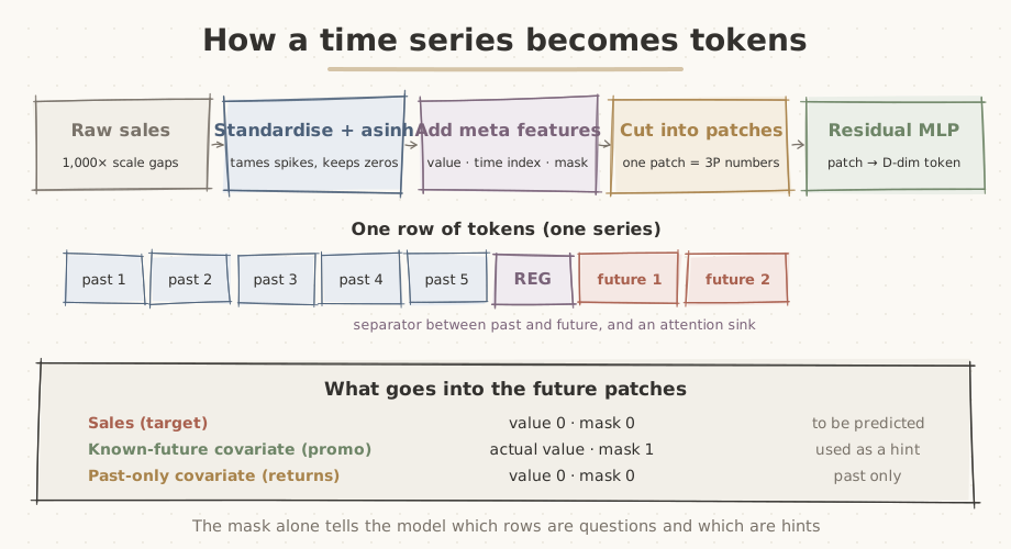
A future sales patch has value 0 and mask 0. The model is trained to fill it in.
2. Laying out one seller as a grid
Once tokenised, one seller’s input becomes a grid. Series run down the side: sales, a promotion flag, the return rate and so on. Patches run across. With V series and N patches, there are V×N tokens.
Information needs to flow in two directions across this grid.
One is within the sales row, from past patches to future ones: how this time last year went, what the recent trend is. The other is at the same patch position, from the promotion row to the sales row: the fact that a promotion is scheduled for next week.
Chronos-2 attends in the two directions separately. Across is time attention. Down is group attention.
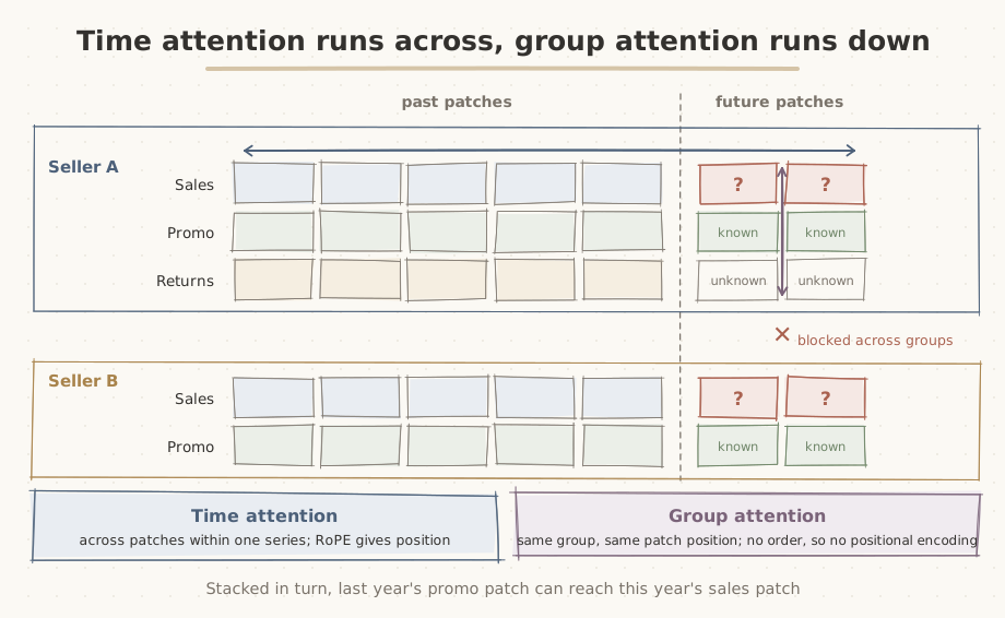
Group attention only flows within a group. Seller A’s covariates never leak to seller B.
3. Time attention
Time attention is the familiar self-attention. The N patches of one series attend to each other. Lay the grid out as (series, patches, D), treat the series axis as the batch, and you are done.
class TimeAttention(nn.Module):
    """Within one series, across its patches"""
    def __init__(self, d, h):
        super().__init__()
        self.norm = nn.LayerNorm(d)
        self.attn = nn.MultiheadAttention(d, h, batch_first=True)

    def forward(self, x):                   # x: (S, N, D)
        y = self.norm(x)
        return x + self.attn(y, y, y, need_weights=False)[0]   # the real model applies RoPE here
There is no causal mask.
Chronos-2 is encoder-only, so past patches see future patches and future patches see past ones.
Doesn’t something leak? No, because the future sales patches are empty. If anything, covariate information in the forecast window gets a path to spread back into the past.
Position comes from RoPE (rotary position embedding), which I left out of the code above to keep only the core.
4. Group attention
Group attention looks at the grid rotated. Fix one patch position and attend across the series in the same group at that position. Seller A’s second sales patch looks at seller A’s second promotion patch and second return-rate patch.
The interesting part of the implementation is that groups come in different sizes. One seller has three covariates, another has ten.
You could pad every group to the same size, but Chronos-2 takes another route. It flattens every series in the batch into one list, attaches a group ID to each series, and turns those IDs into a 2D mask.
With group IDs [0, 0, 0, 1, 1], the first three see only each other and the last two see only each other: a block-diagonal mask.
class GroupAttention(nn.Module):
    """Across series in the same group, at the same patch position"""
    def __init__(self, d, h):
        super().__init__()
        self.norm = nn.LayerNorm(d)
        self.attn = nn.MultiheadAttention(d, h, batch_first=True)

    def forward(self, x, group_ids):        # x: (S, N, D), group_ids: (S,)
        y = self.norm(x).transpose(0, 1)    # (N, S, D): one row of series per patch position
        blocked = group_ids[:, None] != group_ids[None, :]   # (S, S), True = may not attend
        y = self.attn(y, y, y, attn_mask=blocked, need_weights=False)[0]
        return x + y.transpose(0, 1)
A single transpose swaps the axes, and that is all. The series axis, which was the batch in time attention, becomes the sequence here, and the patch axis becomes the batch.
There is no positional encoding.
Series in a group have no order, so whether sales is the first row or the third, the result must be the same.
It is easy to check that the mask really blocks. I set group IDs to [0, 0, 1, 1, 1], shook group 1’s inputs hard, and ran the block. Group 1’s outputs moved by nearly 16. Group 0’s outputs moved by exactly 0.
Not a trace of seller B’s data reaches seller A’s forecast.
Alternate the two kinds of attention and you have a block.
class Block(nn.Module):
    def __init__(self, d, h):
        super().__init__()
        self.time = TimeAttention(d, h)
        self.group = GroupAttention(d, h)
        self.ff = nn.Sequential(nn.LayerNorm(d), nn.Linear(d, 4 * d),
                                nn.GELU(), nn.Linear(4 * d, d))

    def forward(self, x, group_ids):
        x = self.time(x)
        x = self.group(x, group_ids)
        return x + self.ff(x)
5. Why not attend across the whole grid at once
Why not flatten the V×N tokens into one sequence and let everything attend to everything?
Because the cost grows to (V·N)².
Moirai-1 did flatten multivariate inputs this way, and the Chronos-2 paper notes that this limits scalability when there are many variables.
Split across and down, and time attention costs V·N² while group attention costs N·V², which is far cheaper.
It is the same idea image models call axial attention.
The numbers make it concrete. Two years of daily sales, a 90-day horizon and patches of 16 give an N of about 52. With sales plus nine covariates, V is 10, and full attention has 270,000 attending pairs. Split, it has 32,000, about eight times fewer.
Group one seller’s 50 products together (V=50) and the gap widens to 6.76 million pairs against 265,000, twenty-five times.
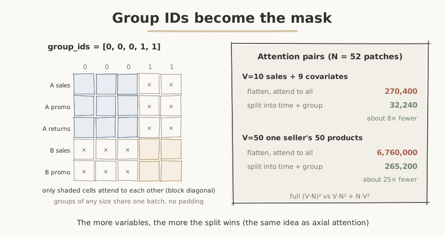
The more variables, the more the split wins.
It might seem you lose something by splitting, but stacking the two in turn lets information flow diagonally. Getting from the promotion row’s next-month patch to the sales row’s next-month patch takes one group attention.
Getting from last year’s promotion patch to this year’s sales patch takes two moves: cross via group attention, then travel via time attention. That is why the blocks are stacked.
6. How covariates get in
With group attention in place, adding covariates turns out to be surprisingly simple. A covariate is just another series in the same group. The only difference is whether it has values in the forecast window.
Sales have values only in the past, with mask 0 in the future. Past-only covariates (return rate, rating) are mask 0 in the future too. Known-future covariates (promotion schedule, holidays) are filled into the forecast window with mask 1. The model reads the mask and works out what each row is.
The remaining details: with a single target, categorical covariates are target-encoded into numbers and fed in the same way. Loss is computed only on the sales row’s future patches, and predictions for covariate rows are discarded. Twenty-one quantiles from 0.01 to 0.99 come out at once.
To see whether this really works, I ran a small experiment. Sales got weekly seasonality, and on promotion days they were 2.5 times higher. The promotion schedule was given as a covariate known into the future. A small model built from two of the blocks above (embedding size 64) trained for 600 steps on CPU.
| Setup | Quantile loss (normalised) | Share of actuals below P10 |
|---|---|---|
| No group (sales alone) | 0.091 | 12.5% |
| Sales and promotion in one group | 0.029 | 9.3% |
Same model, same data, different group IDs.
Alone, the sales series has no way to know about next week’s promotion.
So it forecasts every day about the same and spreads its uncertainty wide. In the same group, it picks up the promotion patches and pinpoints the days sales jump. Loss fell to about a third, and P10 coverage came close to the 10% target.
Full experiment code (PyTorch, under a minute on CPU)
import math, torch, torch.nn as nn

def robust_scale(x, obs):
    n = obs.sum(-1, keepdim=True).clamp_min(1)
    mu = (x * obs).sum(-1, keepdim=True) / n
    sd = ((((x - mu) * obs) ** 2).sum(-1, keepdim=True) / n).sqrt().clamp_min(1e-6)
    return torch.asinh((x - mu) / sd), mu, sd

class PatchEmbed(nn.Module):
    def __init__(self, P, d):
        super().__init__()
        self.lin = nn.Linear(3 * P, d)
        self.mlp = nn.Sequential(nn.Linear(3 * P, d), nn.GELU(), nn.Linear(d, d))
    def forward(self, v, t, m, P):
        S, L = v.shape
        x = torch.cat([a.reshape(S, L // P, P) for a in (v, t, m)], -1)
        return self.lin(x) + self.mlp(x)

class TimeAttention(nn.Module):
    def __init__(self, d, h):
        super().__init__()
        self.norm, self.attn = nn.LayerNorm(d), nn.MultiheadAttention(d, h, batch_first=True)
    def forward(self, x):
        y = self.norm(x)
        return x + self.attn(y, y, y, need_weights=False)[0]

class GroupAttention(nn.Module):
    def __init__(self, d, h):
        super().__init__()
        self.norm, self.attn = nn.LayerNorm(d), nn.MultiheadAttention(d, h, batch_first=True)
    def forward(self, x, group_ids):
        y = self.norm(x).transpose(0, 1)
        blocked = group_ids[:, None] != group_ids[None, :]
        y = self.attn(y, y, y, attn_mask=blocked, need_weights=False)[0]
        return x + y.transpose(0, 1)

class Block(nn.Module):
    def __init__(self, d, h):
        super().__init__()
        self.time, self.group = TimeAttention(d, h), GroupAttention(d, h)
        self.ff = nn.Sequential(nn.LayerNorm(d), nn.Linear(d, 4 * d), nn.GELU(), nn.Linear(4 * d, d))
    def forward(self, x, group_ids):
        x = self.time(x)
        x = self.group(x, group_ids)
        return x + self.ff(x)

class Tiny(nn.Module):
    def __init__(self, P=8, d=64, h=4, n_blocks=2, qs=(0.1, 0.5, 0.9)):
        super().__init__()
        self.P, self.qs = P, torch.tensor(qs)
        self.embed = PatchEmbed(P, d)
        self.blocks = nn.ModuleList(Block(d, h) for _ in range(n_blocks))
        self.head = nn.Sequential(nn.LayerNorm(d), nn.Linear(d, P * len(qs)))
    def forward(self, v, t, m, group_ids):
        x = self.embed(v, t, m, self.P)
        for b in self.blocks:
            x = b(x, group_ids)
        return self.head(x)

def pinball(pred, y, qs):
    d = y.unsqueeze(-1) - pred
    return torch.maximum(qs * d, (qs - 1) * d).mean()

T, H, P = 64, 16, 8   # 64 days of history, 16-day horizon, patch 8

def make_batch(B):
    t = torch.arange(T + H).float()
    base = 100 * (1 + 0.3 * torch.sin(2 * math.pi * t / 7))       # weekly seasonality
    promo = (torch.rand(B, T + H) < 0.15).float()                 # promotions known into the future
    level = torch.exp(torch.randn(B, 1))                          # every seller has a different scale
    y = level * base * (1 + 1.5 * promo) * torch.exp(torch.randn(B, T + H) * 0.1)
    return y, promo

def to_inputs(y, promo, use_group):
    B = y.shape[0]
    tgt_obs = torch.cat([torch.ones(B, T), torch.zeros(B, H)], 1)  # hide the future of sales
    cov_obs = torch.ones(B, T + H)                                 # the promotion's future is visible
    zt, mu, sd = robust_scale(y[:, :T], tgt_obs[:, :T])
    zt = torch.cat([zt, torch.zeros(B, H)], 1)
    zc, pm, ps = robust_scale(promo[:, :T], cov_obs[:, :T])
    zc = torch.cat([zc, torch.asinh((promo[:, T:] - pm) / ps)], 1)
    v = torch.stack([zt, zc], 1).reshape(2 * B, T + H)            # as [sales, promotion] pairs
    m = torch.stack([tgt_obs, cov_obs], 1).reshape(2 * B, T + H)
    tix = ((torch.arange(T + H) - T) / 2048.0).expand(2 * B, -1)  # the forecast start is 0
    g = torch.arange(B).repeat_interleave(2) if use_group else torch.arange(2 * B)
    return v, tix, m, g, mu, sd

def run(use_group, steps=600, B=64):
    torch.manual_seed(1)
    model = Tiny(P=P)
    opt = torch.optim.AdamW(model.parameters(), 3e-3)
    for _ in range(steps):
        y, promo = make_batch(B)
        v, tix, m, g, mu, sd = to_inputs(y, promo, use_group)
        out = model(v, tix, m, g)[0::2, T // P:].reshape(B, H, 3)  # only the sales rows' future patches
        loss = pinball(out, torch.asinh((y[:, T:] - mu) / sd), model.qs)
        opt.zero_grad(); loss.backward(); opt.step()
    torch.manual_seed(123)
    with torch.no_grad():
        y, promo = make_batch(2048)
        v, tix, m, g, mu, sd = to_inputs(y, promo, use_group)
        out = model(v, tix, m, g)[0::2, T // P:].reshape(2048, H, 3)
        pred = mu.unsqueeze(-1) + sd.unsqueeze(-1) * torch.sinh(out)
        wql = pinball(pred, y[:, T:], model.qs).item() / y[:, T:].abs().mean().item()
        below_p10 = (y[:, T:] < pred[..., 0]).float().mean().item()
    return wql, below_p10

for use_group in (False, True):
    wql, below = run(use_group)
    print(f"group={use_group}: quantile loss {wql:.3f}, below P10 {below:.1%}")
It also follows that how you group things defines the task.
The Chronos-2 paper gives four kinds of group: a single series (univariate), series sharing a source or metadata (cross-learning), variables with shared dynamics (multivariate), and a target with its covariates (covariate-aware forecasting).
For sales, a seller plus their covariates as one group is the default. You could also group one seller’s products, or sellers in the same category.
That last option is especially useful for new sellers. Leave a seller with two or three months of history on their own and the forecast is weak. Put them in a group with similar sellers from the same category and they borrow those sellers’ patterns, a bit like a new pupil guessing the day’s timetable from their classmates.
In its conclusion, the Chronos-2 paper names retrieval-augmented forecasting as a future direction: finding similar series through metadata or embeddings and grouping them. The caveat is that mixing in unrelated sellers only adds noise.
7. Daily quantiles don’t add up to a monthly one
Loan limits are usually set on a 30- or 90-day total. But Chronos-Bolt and Chronos-2 output a separate quantile for each time step.
So is the P10 of a 30-day total the sum of the daily P10s?
No. I simulated a seller with median daily sales of ₩1M. If days are uncorrelated, summing the daily P10 over 30 days gives ₩13.9M, while the true P10 of the 30-day total is ₩30.6M. More than half too low.
Even with a day-to-day correlation of 0.8 it is 40% low, and at 0.95 it is still 20% low. Set limits this way and you systematically under-lend.
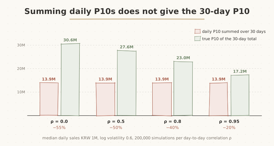
The lower the day-to-day correlation, the bigger the gap.
Summing every daily P10 amounts to assuming a bad day every single day for 30 days, like working out a month’s income as if every day were your worst. In reality bad days and good days mix, and the total swings less. Summing P90s overshoots the other way.
So if the forecast is for a limit, make the target the total over the period you need from the start. Feed in weekly or monthly aggregates and predict quantiles of that total directly.
Alternatively, use a model that samples multiple future paths, like the first Chronos. Sum each path and read quantiles off that distribution. With a model that only outputs per-step quantiles, the first option is the only one.
8. Other things to watch
Known-future covariates must really be known
Only put into the forecast window what you can actually know at underwriting time. Promotions already scheduled and public holidays are fine. Actual ad spend and actual visitor numbers are not.
In a backtest, mixing these in just makes performance look good, which is why it is hard to catch. It is a common leak in lending models, and the only defence is to ask of every feature whether you would know its value on the day of the decision.
For sellers with many zeros, start with the aggregation level
asinh scaling can handle zeros. But a seller with more zero days than sales days gives the model little to look at when fed daily.
Aggregating weekly reduces the zeros and brings the pattern back. If limits are monthly there is no need to forecast daily anyway, and it solves the summing problem from section 7 as well.
Evaluate the coverage of the quantile you’ll use
Run a rolling backtest, moving the cutoff date several times. Alongside overall metrics like quantile loss, check the coverage of the quantile used for limits separately.
If limits are set at P10, one number matters most.
Does the share of actual sales falling below P10 sit near 10%? As the LightGBM experiment in part one showed, this drifts easily when the period changes, so a calibration step on recent data is a good idea.
Start the comparison zero-shot
A pretrained model can run with no training at all. Put LightGBM and zero-shot Chronos-2 through the same backtest and see which wins where, by seller segment (history length, scale, intermittency). Fine-tuning can wait until you have seen the gap.
Chronos-2 has 120 million parameters and runs on a single mid-range GPU. The small 28-million-parameter version reportedly loses little accuracy while running nearly twice as fast.
9. A personal view
What I found most interesting about group attention is that covariate-aware forecasting, multivariate forecasting and cross-learning turn out to be the same operation. The three have long been studied as separate problems. In Chronos-2, only the group IDs differ.
The architecture stays the same, and what you put in the same group defines the task.
That moves much of what used to be model design into deciding how to group the data. Which covariates are truly known in advance. Which sellers resemble each other. How many days of total the limit needs. A pretrained model won’t tell you any of that.
In the end, how you fill in that one line of group_ids probably changes the result more than how many layers you stack. And that line is filled in best by someone who has spent a long time looking at sales data.
Related posts:
- Sales Forecasting (1) From Tree Models to Chronos
- How Do You Grade an LLM? Eleven Evaluation Methods, Sorted into Four Families
References
- Chronos-2: From Univariate to Universal Forecasting (Ansari et al., 2025)
- Chronos: Learning the Language of Time Series (Ansari et al., 2024)
- A Time Series is Worth 64 Words: Long-term Forecasting with Transformers (PatchTST, Nie et al., 2023)
- Axial Attention in Multidimensional Transformers (Ho et al., 2019)
- Unified Training of Universal Time Series Forecasting Transformers (Moirai, Woo et al., 2024)
- chronos-forecasting (GitHub)
Written as of 30 September 2026 from the Chronos-2 technical report. The code keeps only the core to explain the structure and differs from the real implementation (RoPE, the REG token, residual block details). The group isolation check, the toy experiment and the quantile-summing simulation are all my own runs, and the figures will differ on real seller data.